Name: _________________________________________
In this lab assignment, you will explore two common uses of computer technology in scientific research: data visualization and system modeling. The discipline you will consider is biology, specifically the study of population growth in a predator-prey relationship.
Since the amount of real-world data that can be collected in domains such this may be massive, computers are essential for storing, accessing, and analyzing the patterns inherent in the data. Often, being able to visualize the data can allow a scientist to see patterns and draw conclusions that would otherwise be difficult to discern. In the first part of this lab, you will use a program to graph population statistics taken over a 60 year period and look for patterns that link the predator-prey populations.
When studying complex systems, such as an ecosystem involving predator and prey species, simply collecting and analyzing real-world data is sometimes not enough. To further study the system and perhaps test hypotheses about its behavior, scientists often develop computer models of the system. Computer models allow the scientist to alter the parameters of the system and observe the resulting changes. And since computers are fast, long-range developments in the system can be simulated at incredible speeds, at a fraction of the cost of field observation. In the second part of this lab, you will use a computer model to study the predator-prey relationship.
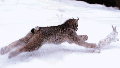
A classic example of the predator-prey relationship in nature involves the Canada lynx and the snowshoe hare. The Canada lynx ranges across upper North America and preys almost exclusively on snowshoe hare. Starting in the mid 1800's, the Hudson's Bay Company tracked the number of lynx and hare pelts obtained by trappers (see the tables below from szukaitas.com). Assuming that these numbers provide a proportional estimate of the two populations over time, scientists have used this data to chart the predator-prey relationships between the lynx and hare.
|
|
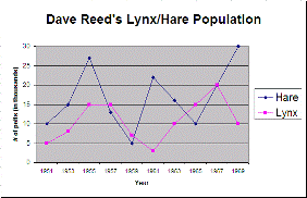
EXERCISE 1: Graph the pelt data using an application such as Microsoft Excel. Your graph should plot the numbers of pelts, clearly identifying which set of data is which and labeling the axes appropriately. The graph should also have your name included in the title. If you are not familiar with Excel or some other graphing program (e.g., GraphPad), we will go over the basics of graphing in Excel in class. For example, the following graph provides a sample (using fictional data):Once you have completed your graph, describe the pattern (if any) exhibited by that graph. Does there appear to be a cyclic pattern to the growth and decline of the populations? If so, is the cycle length consistent? Are the growth/decline patterns of the two populations identical, or are they linked in some way? What do you think the pattern of the graph suggests about the predator/prey relationship between the two populations?
EXERCISE 2: Save the pelt table and graph in a Web page. If you are using Excel, a simple way to do this is just to go to "Save As" under the File menu, and select "Web Page (*.htm, *.html)" as the file type before saving. This will create a Web page with an accompanying folder of support documents.Copy both the Web page and the accompanying support folder to your personal Web space on the people server, and add a link to your home page that will connect to this new page. For example, click here to see my sample page.
EXERCISE 3: In recent decades, scientists have revisited the common interpretation of the lynx-hare population data, i.e., that the population cycles were primarily attributable to the predator-prey relationship. While the predator-prey relationship undoubtedly contributes to the pattern, it has been proposed that other factors may be of equal or even greater importance. Conduct some research (either online or through other sources) and cite another factor that could significantly contribute to the observed population pattern. Be sure to list your source.
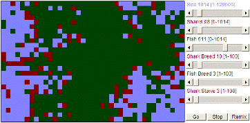 Various computer models have been created to simulate the predator-prey relationship
within an ecosystem. The
WATOR simulation was one of the first
of these. It models a predator-prey relationship, described in terms of sharks and
fish (although these could also be thought of as lynx and hares). The simulator
allows the user to adjust the basic characteristics of the two species. For example,
the default breeding period for fish in the simulation is 3, meaning that a newborn
fish requires 3 units of time before it is able to reproduce. By default, sharks have
a longer breeding period of 10 units of time, and will starve to death if they do
not obtain food within 3 units of time. Given these characteristics, the WATOR simulator
models the growth and decline of the populations over time, displaying the species
as different colored squares on the ecosystem grid.
Various computer models have been created to simulate the predator-prey relationship
within an ecosystem. The
WATOR simulation was one of the first
of these. It models a predator-prey relationship, described in terms of sharks and
fish (although these could also be thought of as lynx and hares). The simulator
allows the user to adjust the basic characteristics of the two species. For example,
the default breeding period for fish in the simulation is 3, meaning that a newborn
fish requires 3 units of time before it is able to reproduce. By default, sharks have
a longer breeding period of 10 units of time, and will starve to death if they do
not obtain food within 3 units of time. Given these characteristics, the WATOR simulator
models the growth and decline of the populations over time, displaying the species
as different colored squares on the ecosystem grid.
EXERCISE 4: Go to the WATOR Simulation Web site and observe the simulation of the predator-prey relationship. What color square is used to represent a shark in the simulation? What color is used for a fish? How did you determine this?
Describe the behavior of the simulation. What behavior does the ecosystem grid exhibit over time? Below the grid, the simulation graphs the populations as they grow and decline. Does the running graph of the shark/fish populations resemble the lynx/hare graph you constructed? Justify your answers.
EXERCISE 5: How sensitive is the WATOR simulation to the initial populations of sharks and fish in the environment? If you decrease one of the populations by 50%, would you expect it to change the overall behavior of the simulation in the long run? Write your hypothesis below, along with a short rationale, before testing it in the simulator.
Now, test your hypothesis by stopping the simulation, manually adjusting the population, and then observing whether the resulting behavior supports or refutes your claim. Be sure to run several simulations, as randomness can skew the results on occasion. Describe your results.
EXERCISE 6: How sensitive is the WATOR simulation to changes in the breeding rates of the two populations? Which, if either, population would have the greater impact if it was changed: shark breeding or fish breeding? Write your hypothesis below, along with a short rationale, before testing it in the simulator.
Now, test your hypothesis by stopping the simulation, manually adjusting the breeding rates, and then observing whether the resulting behavior supports or refutes your claim. Be sure to run several simulations, as randomness can skew the results on occasion. Describe your results.
Is there a point at which adjusting the breeding rates leads to extinction of one or both populations? If so, identify when that occurs (answers may be approximate).
EXERCISE 7: How sensitive is the WATOR simulation to changes in the starvation rate of sharks? Write your hypothesis below, along with a short rationale, before testing it in the simulator.
Now, test your hypothesis by stopping the simulation, manually adjusting the starvation rate, and then observing whether the resulting behavior supports or refutes your claim. Be sure to run several simulations, as randomness can skew the results on occasion. Describe your results.
Is there a point at which adjusting the starvation rate leads to extinction of one or both populations? If so, identify when that occurs (answers may be approximate).
EXERCISE 8: It must always be remembered that simulations are simplifications of real-world systems. When a scientist models a complex system, he or she makes decisions about which factors are important and which can be ignored. Sometimes, these ignored factors turn out to be important, limiting the effectiveness of the model in capturing the real-world behavior.Consider the predator-prey relationship that is being modeled in the WATOR simulator. Describe at least one factor in such a real-world relationship that is being ignored in the simulation. Do you think that this factor significantly limits the model in terms of its ability to simulate the real-world system? Explain your answer.
EXERCISE 9: Using the Internet or other references, identify another example where computer simulations were used to study natural population growth patterns. Briefly describe how the simulation allowed researchers to learn something new about the nature of the underlying organisms and/or ecosystem. Be sure to list your sources.